Chapter 9
Summarizing and Graphing Your Data
IN THIS CHAPTER
 Representing categorical data
Characterizing numerical variables
Putting numerical summaries into tables
Displaying numerical variables with bars and graphs
A large study can involve thousands of participants, hundreds of variables, and millions of individual data points. You need to summarize this ocean of individual values for each variable down to a few numbers, called summary statistics, that give readers an idea of what the whole collection of numbers looks like — that is, how they’re distributed.
When presenting your results, you usually want to arrange these summary statistics into tables that describe how the variables change over time or differ between categories, or how two or more variables are related to each other. And, because a picture really is worth a thousand words, you will want to display these distributions, changes, differences, and relationships graphically. In this chapter, we show you how to summarize and graph both categorical and numerical data. Note: This chapter doesn’t cover time-to-event (survival) data, which is the topic of Chapter 22.
Summarizing and Graphing Categorical Data
A categorical variable is summarized by tallying the number of participants in each category and expressing this number as a count. You might also compute a percentage of the total number of participants in all categories combined. So a sample of 422 participants can be summarized by health insurance type, as shown in Table 9-1.
TABLE 9-1 Study Participants Categorized by Health Insurance Type
Health Insurance Type |
Count |
Percent of Total |
|---|---|---|
Commercial |
128 |
30.3% |
Public |
141 |
33.4% |
Military |
70 |
16.6% |
Other |
83 |
19.7% |
Total |
422 |
100% |
The joint distribution of participants between two categorical variables is summarized by a cross-tabulation (or cross-tab). Table 9-2 shows an example of a cross-tab of the same participants in our example with type of health insurance on one axis, and urban-rural classification of their residence on the other.
TABLE 9-2 Cross-Tabulation of Participants by Two Categorical Variables
Health Insurance Type |
||||||
|---|---|---|---|---|---|---|
Commercial |
Public |
Military |
Other |
Total |
||
Urban-Rural Classification of Residence |
Rural |
60 |
60 |
34 |
42 |
196 |
Urban |
68 |
81 |
36 |
41 |
226 |
|
Total |
128 |
141 |
70 |
83 |
422 |
|
After looking at the frequencies in Table 9-2, you may be curious about the percentages, which would make these numbers more comparable. But a cross-tab can get very cluttered if you try to include them, as there are different types: the column percentage, the row percentage, and the total percentage. For example, the 60 rural residents with commercial health insurance in Table 9-2 comprise 46.9 percent of all participants with commercial health insurance, because 60 divided by the total number with commercial health insurance, which is 128 (the column total), equals 46.9 percent.
Groups are often compared across columns, and if that is the intention, column percentages should be displayed. But if you divide these same 60 rural residents with commercial insurance by their row total of 169 rural residents, you find they make up 30.6 percent of all rural residents, which is a row percentage. And if you go on to divide these 60 participants by the total sample size of the study, which is 422, you find that they make up 14.2 percent of all participants in the study.
Categorical data are typically displayed graphically as frequency bar charts and as pie charts:
- Frequency bar charts: Displaying the spread of participants across the different categories of a variable is commonly done by a bar chart (see Figure 9-1a). Generally, statistical programs are used to make bar charts. To create a bar chart manually from a tally of participants in each category, you draw a graph containing one vertical bar for each category, making the height proportional to the number of participants in that category.
- Pie charts: Pie charts indicate the relative number of participants in each category by the angle of a circular wedge, which can also be considered more deliciously as a piece of the pie. To create a pie chart manually, you multiply the percentage of participants in each category by 360, which is the number of degrees of arc in a full circle, and then divide by 100. By doing that, you are essentially figuring out what proportion of the circle to devote to that pie piece. Next, you draw a circle with a compass, and then split it up into wedges using a protractor — remember from high school math? Trust us, it’s easier to use statistical software.
 Most scientific writers recommend the usage of bar charts over pie charts. They express more information in a smaller space, and allow for more accurate visual comparisons.

© John Wiley & Sons, Inc.
FIGURE 9-1: A frequency bar chart (a) and pie chart (b).
Summarizing Numerical Data
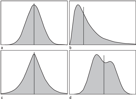
Summarizing a numerical variable isn’t as simple as summarizing a categorical variable. The summary statistics for a numerical variable should convey how the individual values of that variable are distributed across your sample in a concise and meaningful way. These summary statistics should give you some idea of the shape of the true distribution of that variable in the population from which you draw your sample (read Chapter 3 and Chapter 6 to refresh your memory about sampling). That true population distribution can have almost any shape, including the typical shapes shown in Figure 9-2: normal, skewed, pointy-topped, and bimodal (two-peaked).
© John Wiley & Sons, Inc.
FIGURE 9-2: Four different shapes of distributions: normal (a), skewed (b), pointy-topped (c), and bimodal (two-peaked) (d).
How can you convey a visual picture of what the true distribution may look like by using just a few summary numbers? By reporting values of measures of some important characteristics of these distributions, so that the reader can infer the shape. This is similar to learning that one Olympic ice skater scored an average of 9.0 compared to another who scored an average of 5.0. You will not know what the skate routines looked like unless you watch them, but the score will already tell you that if you were to watch them, you would expect to see that the one that scored 9.0 was executed in a more visually pleasing way than the one that scored 5.0.
Frequency distributions have names for their important characteristics, including:
- Center: Where along the distribution of the values do the numbers tend to center?
- Dispersion: How much do these numbers spread out?
- Symmetry: If you were to draw a vertical line down the middle of the distribution, does the distribution shape appear as if the vertical line is a mirror, reflecting an identical shape on both sides? Or do the sides look noticeably different — and if so, how?
- Shape: Is the top of the distribution nicely rounded, or pointier, or flatter?
Like using average skating scores to describe the visual appeal of an Olympic skate routine, to describe a distribution you need to calculate and report numbers that measure each of these four characteristics. These characteristics are what we mean by summary statistics for numerical variables.
Locating the center of your data
When you start exploring a set of numbers, an important first step is to determine what value they tend to center around. This characteristic is called, intuitively enough, central tendency. Many statistical textbooks describe three measures of central tendency: mean (which is the same as average), median, and mode. You may assume these are the three optimal measures to describe a distribution (because they all begin with m and are easy to remember). But all three have limitations, especially when dealing with data obtained from samples in human research, as described in the following sections.
Arithmetic mean
The arithmetic mean, also commonly called the mean (or the average), is the most familiar and most often quoted measure of central tendency. Throughout this book, whenever we use the two-word term the mean, we’re referring to the arithmetic mean. (There are several other kinds of means besides the arithmetic mean, which we describe later in this chapter.)
 The mean of a sample is often denoted by the symbol m or by placing a horizontal bar over the name of the variable, like
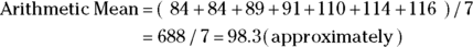
  . The mean is obtained by adding up the values and dividing by the sample size — meaning how many there are. (If you are using software for this, make sure missing values are excluded, or the equation will not compute.) Here’s a small sample of numbers — the diastolic blood pressure (DBP) values of seven study participants (in mmHg) arranged in increasing numerical order: 84, 84, 89, 91, 110, 114, and 116. For the DBP sample:
You can write the general formula for the arithmetic mean of N number of values contained in the variable X in several ways:
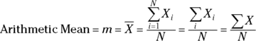
See Chapter 2 for a refresher on mathematical notation and formulas, including how to interpret the various forms of the summation symbol ∑ (the Greek capital sigma). In the rest of this chapter, we use the simplest form, meaning the form without the i subscripts that refer to specific elements of an array, whenever possible.
Some statistical books use the notation such that capital  and capital N refer to census parameters, and lowercase versions of those to refer to sample statistics. In this book, we make it clear each time we present this notation whether we are talking about a census or a sample.
Median
Like the mean, the median is a common measure of central tendency. In fact, it could be argued that the median is the only one of the three that really takes the word central seriously.
The median of a sample is the middle value in the sorted (ordered) set of numbers. By definition, half of the numbers are smaller than the median, and half are larger. The median of a population frequency distribution function (like the curves shown in Figure 9-2) divides the total area under the curve into two equal parts: Half of the area under the curve (AUC) lies to the left of the median, and half lies to the right.
Consider the sample of diastolic blood pressure (DBP) measurements from seven study participants from the preceding section. If you arrange the values in order from lowest to highest mmHg, you can list them as 84, 84, 89, 91, 110, 114, and 116. There are seven values, and 91 is the fourth of the seven sorted values, so that is the median. Three DBPs in the sample are smaller than 91 mmHg, and three are larger than 91 mmHg. If you have an even number of values, the median is the average of the two middle values. So imagine that you add a value of 118 mmHg to the top of your list, so you now have eight values. To get the median, you would make an average of the fourth and fifth value, which would be (91 + 110)/2 = 100.5 mmHg (don’t be thrown off by the 0.5).
Statisticians often say that they prefer the median to the mean because the median is much less strongly influenced by extreme outliers than the mean. For example, if the largest value for DBP had been very high — such as 150 mmHg instead of 116 mmHg — the mean would have jumped from 98.3 mmHg up to 103.1 mmHg. But in the same case, the median would have remained unchanged at 91. Here’s an even more extreme example: If a multibillionaire were to move into a certain state, the mean family net worth in that state might rise by hundreds of dollars, but the median family net worth would probably rise by only a few cents (if it were to rise at all). This is why you often hear the median rather than mean income in reports comparing income across regions.
Mode
The mode of a sample of numbers is the most frequently occurring value in the sample. One way to remember this is to consider that mode means fashion in French, so the mode is the most popular value in the data set. But the mode has several issues when it comes to summarizing the centrality of observed values for continuous numerical variables. Often there are no exact duplicates, so there is no mode. If there are any exact duplicates, they usually are not in the center of the data. And if there is more than one value that is duplicated the same number of times, you will have more than one mode.
So the mode is not a good summary statistic for sampled data. But it’s useful for characterizing a population distribution, because it’s the value where the peak of the distribution function occurs. Some distribution functions can have two peaks (a bimodal distribution), as shown earlier in Figure 9-2d, indicating two distinct subpopulations, such as the distribution of age of death from influenza in many populations, where we see a mode in young children, and another mode in older adults.
Considering some other “means” to measure central tendency
Several other kinds of means are useful measures of central tendency in certain circumstances. They’re called means because they all calculated using the same approach. The difference is that each type of mean adds a slightly different twist to the basic mathematical process.
INNER MEAN
The inner mean (also called the trimmed mean) of N numbers is calculated by removing the lowest value (the minimum) and the highest value (the maximum), and calculating the arithmetic mean of the remaining N – 2 inner values. For the sample of seven values of DBP from study participants from the example used earlier in this chapter (which were 84, 84, 89, 91, 110, 114, and 116 mmHg), you would drop the minimum and the maximum to compute the inner mean:  .
.
An inner mean that is even more inner can be calculated by making an even stricter rule. The rule could be to drop the two (or more) of the highest and two (or more) of the lowest values from the data, and then calculate the arithmetic mean of the remaining values. In the interest of fairness, you should always chop the same number of values from the low end as from the high end. Like the median (discussed earlier in this chapter), the inner mean is more resistant to extreme values called outliers than the arithmetic mean.
GEOMETRIC MEAN
The geometric mean (often abbreviated GM) can be defined by two different-looking formulas that produce exactly the same value. The basic definition has this formula:

We describe the product symbol Π (the Greek capital pi) in Chapter 2. This formula is telling you to multiply the values of the N observations together, and then take the Nth root of the product. Using the numbers from the earlier example (where you had DBP data on seven participants, with the values 84, 84, 89, 91, 110, 114, and 116 mmHg), the equation looks like this:

Even with technology, this formula is computationally challenging. By using logarithms (which turn multiplications into additions and roots into divisions), you can develop a numerically stable alternative formula, which is:
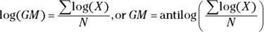
This formula may look complicated, but it really just says, “The geometric mean is the antilog of the mean of the logs of the values in the sample.” In other words, to calculate the GM using this formula, you take the log of each value in your sample, then average all those logs together, and then take the antilog of that average. You can choose to use either natural or common logarithms, but make sure that whatever you choose, you use same type of antilog. (Flip to Chapter 2 for the basics of logarithms.)
Describing the spread of your data
After central tendency (described earlier in “Locating the center of your data”), the second most important set of summary statistics for numerical values refers to how tightly or loosely they tend to cluster around a central value, meaning how they are dispersed. There are several common measures of dispersion, as you find out in the following sections.
Standard deviation, variance, and coefficient of variation
The standard deviation (usually abbreviated SD, sd, or just s) of a set of numerical values tells you how much the individual values tend to differ from the mean in either direction (see “Locating the center of your data” for a discussion of the mean). The SD is calculated as follows:
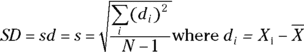
This formula is saying that you calculate the SD of a set of N numbers by first subtracting the mean from each value ( ) to get the deviation (
 ) of each value from the mean. Then, you take the square each of these deviations and add up the
  terms. After that, you divide that number by N – 1, and finally, you take the square root of that number to get your answer, which is the SD.
For the sample of diastolic blood pressure (DBP) measurements for seven study participants in the example used earlier in this chapter, where the values are 84, 84, 89, 91, 110, 114, and 116 mmHg and the mean is 98.3 mmHg, you calculate the SD as follows:

Several other useful measures of dispersion are related to the SD:
- Variance: The variance is just the square of the SD. For the DBP example, the variance
 .
. - Coefficient of variation: The coefficient of variation (CV) is the SD divided by the mean. For the DBP example,
 percent.
Range
The range of a set of values is the minimum value subtracted from the maximum value:

Consider the example from the preceding section, where you had DBP measurements from seven study participants (which were 84, 84, 89, 91, 110, 114, and 116 mmHg). The minimum value is 84, the maximum value is 116, and the range is 32 (equal to  ).
).
Centiles
The basic idea of the median is that ½ (half) of your numbers are less than the median, and the other ½ are greater than the median. This concept can be extended to other fractions besides ½.
A centile (also referred to as percentile) is a value that a certain percentage of the values are less than. For example, ¼ of the values are less than the 25th centile (and ¾ of the values are greater). The median is just the 50th centile. The 25th, 50th, and 75th centiles are called the first, second, and third quartiles, respectively, and are used often. There are other sets of centiles, such as deciles, which break at every ten percentiles, that are used less often.
As we explain in the earlier section “Median,” if the sorted sequence of your numerical variable has no middle value, you have to calculate the median as the average of the two middle numbers. The same situation comes up in calculating centiles, but there are different ways that statistical software does the calculation. Fortunately, the different formulas they use give nearly the same result.
The inter-quartile range (IQR) is the difference between the 25th and 75th centiles (the first and third quartiles).
Numerically expressing the symmetry and shape of the distribution
In the following sections, we discuss two summary statistics used to describe aspects of the symmetry and shape of the distribution of values of numerical variables (pictured earlier in Figure 9-2).
Skewness
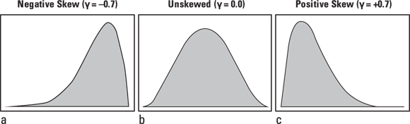
Skewness refers to the left-right symmetry of the distribution. Figure 9-3 illustrates some examples.
© John Wiley & Sons, Inc.
FIGURE 9-3: Distributions can be left-skewed (a), symmetric (b), or right-skewed (c).
Figure 9-3b shows a symmetrical distribution. If you look back to Figures 9-2a and 9-2c, which are also symmetrical, they look like the vertical line in the center is a mirror reflecting perfect symmetry, so these have no skewness. But Figure 9-2b has a long tail on the right, so it is considered right skewed (and if you flipped the shape horizontally, it would have a long tail on the left, and be considered left-skewed, as in Figure 9-3a).
How do you express skewness in a summary statistic? The most common skewness coefficient, often represented by the Greek letter γ (lowercase gamma), is calculated by averaging the cubes (third powers) of the deviations of each point from the mean and scaling by the SD. Its value can be positive, negative, or zero.
Here is how to interpret the skewness coefficient (γ):
- A negative γ indicates left-skewed data (Figure 9-3a).
- A zero γ indicates unskewed data (Figures 9-2a and 9-2c, and Figure 9-3b).
- A positive γ indicates right-skewed data (Figures 9-2b and 9-3c).
Notice that in Figure 9-3a, which is left-skewed, the γ = –0.7, and for Figure 9-3c, which is right-skewed, the γ = 0.7. And for Figure 9-3b — the symmetrical distribution — the γ = 0, but this almost never happens in real life. So how large does γ have to be before you suspect real skewness in your data? A rule of thumb for large samples is that if γ is greater than  , your data are probably skewed.
Kurtosis
Kurtosis is a less-used summary statistic of numerical data, but you still need to understand it. Take a look at the three distributions shown in Figure 9-4, which all have the same mean and the same SD. Also, all three have perfect left-right symmetry, meaning they are unskewed. But their shapes are still very different. Kurtosis is a way of quantifying these differences in shape.

© John Wiley & Sons, Inc.
FIGURE 9-4: Three distributions: leptokurtic (a), normal (b), and platykurtic (c).
A good way to compare the kurtosis of the distributions in Figure 9-4 is through the Pearson kurtosis index. The Pearson kurtosis index is often represented by the Greek letter k (lowercase kappa), and is calculated by averaging the fourth powers of the deviations of each point from the mean and scaling by the SD. Its value can range from 1 to infinity and is equal to 3.0 for a normal distribution. The excess kurtosis is the amount by which k exceeds (or falls short of) 3.
One way to think of kurtosis is to see the distribution as a body silhouette. If you think of a typical distribution function curve as having a head (which is near the center), shoulders on either side of the head, and tails out at the ends, the term kurtosis refers to whether the distribution curve tends to have
- A pointy head, fat tails, and no shoulders, which is called leptokurtic, and is shown in Figure 9-4a (where
 ).
). - An appearance of being normally distributed, as shown in Figure 9-4b (where
 ).
). - Broad shoulders, small tails, and not much of a head, which is called platykurtic. This is shown in Figure 9-4c (where
 ).
).
A very rough rule of thumb for large samples is that if k differs from 3 by more than  , your data have abnormal kurtosis.
Structuring Numerical Summaries into Descriptive Tables
Now you know how to calculate the basic summary statistics that convey the general idea of how a set of numerical values is distributed. So which summary statistics do you report? Generally, you select a few of the most useful summary statistics in summarizing your particular data set, and arrange them in a concise way. Many biostatisticians choose to report N, mean, SD, median, minimum, and maximum, and arrange them something like this:

Consider the example used earlier in this chapter of seven measures of diastolic blood pressure (DBP) from a sample of study participants (with the values of 84, 84, 89, 91, 110, 114, and 116 mmHg), where you calculated all these summary statistics. Remember not to display decimals beyond what were collected in the original data. Using this arrangement, the numbers would be reported this way:
The real utility of this kind of compact summary is that you can place it in each cell of a table to show changes over time and between groups. For example, a sample of systolic blood pressure (SBP) measurements taken from study participants before and after treatment with two different hypertension drugs (Drug A and Drug B) can be summarized concisely, as shown in Table 9-3.
TABLE 9-3 Systolic Blood Pressure Treatment Results
Before Treatment |
After Treatment |
Change |
||||
|---|---|---|---|---|---|---|
Mean ± SD (N) |
Median (min – max) |
Mean ± SD (N) |
Median (min – max) |
Mean ± SD (N) |
Median (min – max) |
|
Drug A |
138.7 ± 10.3 (40) |
139.5 (117 – 161) |
121.1 ± 13.9 (40) |
121.5 (85 – 154) |
-17.6 ± 8.0 (40) |
–17.5 (–34 – 4) |
Drug B |
141.0 ± 10.8 (40) |
143.5 (111 – 160) |
141.0 ± 15.4 (40) |
142.5 (100 – 166) |
-0.1 ± 9.9 (40) |
1.5 (–25 – 18) |
Table 9-3 shows that Drug A tended to lower blood pressure by about 18 mmHg. For Drug A, mean SBP changed from 139 to 121 mmHg from before to after treatment, whereas the Drug B group produced no noticeable change in blood pressure because it stayed around 141 mmHg from pretreatment to post-treatment. All that’s missing are some p values to indicate the significance of the changes over time within each group and of the differences between the groups. We show you how to calculate those in Chapter 11.
Graphing Numerical Data
Displaying information graphically is a central part of interpreting and communicating the results of scientific research. You can easily spot subtle features in a graph of your data that you’d never notice in a table of numbers. Entire books have been written about graphing numerical data, so we only give a brief summary of some of the more important points here.
Showing the distribution with histograms
Histograms are bar charts that show what fraction of the participants have values falling within specified intervals called classes. The main purpose of a histogram is to show you how the values of a numerical value are distributed. This distribution is an approximation of the true population frequency distribution for that variable, as shown in Figure 9-5.
© John Wiley & Sons, Inc.
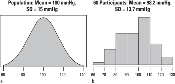
FIGURE 9-5: Population distribution of systolic blood pressure (SBP) measurements in mmHg (a) and distribution of a sample from that population (b).
The smooth curve in Figure 9-5a shows how SBP values are distributed in an infinitely large population. The height of the curve at any SBP value is proportional to the fraction of the population in the immediate vicinity of that SBP. This curve has the typical bell shape of a normal distribution.
The histogram in Figure 9-5b indicates how the SBP measurements of 60 study participants randomly sampled from the population might be distributed. Each bar represents an interval or class of SBP values with a width of ten mmHg. The height of each bar is proportional to the number of participants in the sample whose SBP fell within that class.
Log-normal distributions
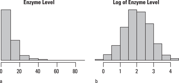
Because a sample is only an imperfect representation the population, determining the precise shape of a distribution can be difficult unless your sample size is very large. Nevertheless, a histogram usually helps you spot skewed data, as shown in Figure 9-6a. This kind of shape is typical of a log-normal distribution (Chapter 25), which is a distribution you often see when analyzing biological measurements, such as lab values. It’s called log-normal because if you take a logarithm (of any type) of each data value, the resulting logs will have a normal distribution, as shown in Figure 9-6b.
© John Wiley & Sons, Inc.
FIGURE 9-6: Log-normal data are skewed (a), but the logarithms are normally distributed (b).
Because distributions are so important to biostatistics, it’s a good practice to prepare a histogram for every numerical variable you plan to analyze. That way, you can see whether it’s noticeably skewed and, if so, whether a logarithmic transformation makes the distribution normal enough so you can use statistics intended for normal distributions on your data.
If you can’t find any transformation that makes your data look even approximately normal, then you have to analyze your data using nonparametric methods, which don’t assume that your data are normally distributed.
Summarizing grouped data with bars, boxes, and whiskers
Sometimes you want to show how a numerical variable differs from one group of participants to another. For example, blood levels of a certain cardiovascular enzyme vary among the cardiology patients at four different clinics: Clinic A, B, C, and D. Two types of graphs are commonly used for this purpose: bar charts and box-and-whiskers plots.
Bar charts
One simple way to display and compare the means of several groups of data is with a bar chart, like the one shown in Figure 9-7a. Here, the bar height for each group of patients equals the mean (or median, or geometric mean) value of the enzyme level for patients at the clinic represented by the bar. And the bar chart becomes even more informative if you indicate the spread of values for each clinical sample by placing lines representing one SD above and below the tops of the bars, as shown in Figure 9-7b. These lines are always referred to as error bars, which is an unfortunate choice of words that can cause confusion when error bars are added to a bar chart. In this case, error refers to statistical error (described in Chapter 6).

© John Wiley & Sons, Inc.
FIGURE 9-7: Bar charts showing mean values (a) and standard deviations (b).
But even with error bars, a bar chart still doesn’t provide a picture of the distribution of enzyme levels within each group. Are the values skewed? Are there outliers? Imagine that you made a histogram for each subgroup of patients — Clinic A, Clinic B, Clinic C, and Clinic D. But if you think about it, four histograms would take up a lot of space. There is a solution for this! Keep reading to find out what it is.
Box-and-whiskers charts
The box-and-whiskers plot (or B&W, or just box plot) plot uses very little space to display a lot of information about the distribution of numbers in one or more groups of participants. A box plot of the same enzyme data used in Figure 9-7 is shown in Figure 9-8a.

© John Wiley & Sons, Inc.
FIGURE 9-8: Box-and-whiskers charts: no-frills (a) and with variable width and notches (b).
Looking at Figure 9-8a, you notice the box plot for each group has the following parts:
- A box spanning the interquartile range (IQR), extending from the first quartile of the variable to the third quartile, thus encompassing the middle 50 percent of the data.
- A thick horizontal line, drawn at the median, which is also the 50th centile. If this falls in the middle of the box, your data are not skewed, but if it falls on either side, be on the lookout for skewness.
- Lines called whiskers extending out to the farthest data point that’s not more than 1.5 times the IQR away from the box, and terminate with a horizontal bar on each side.
- Individual points lying outside the whiskers, which are considered outliers.
Box plots provide a useful visual summary of the distribution of each subgroup for comparison, as shown in Figure 9-8a. As mentioned earlier, a median that’s not located near the middle of the box indicates a skewed distribution.
 Some software draws the different parts of a box plot according to different rules, so you should always check your software’s documentation before you present a box plot so you can describe your box plot accurately.
Software can provide various enhancements to the basic box plot. Figure 9-8b illustrates two such embellishments you may consider using:
- Variable width: The widths of the bars can be scaled to indicate the relative size of each group.
- Notches: The box can have notches that indicate the uncertainty in the estimation of the median. If two groups have non-overlapping notches, they probably have significantly different medians.
Depicting the relationships between numerical variables with other graphs
We started this chapter by developing summary statistics and making graphs of one numeric variable at a time. One example was where we took seven measurements of diastolic blood pressure (DBP) from a group of study participants and developed summary statistics. This is called a univariate analysis because it only concerns one variable. But in the example of box plots in the preceding section, we conducted a bivariate analysis because we were looking at the relationship between two variables in a sample of patients from four different clinics. The two variables were enzyme levels, and source clinic (Clinic A, B, C, or D). We could have done another bivariate analysis looking at two continuous variables (such as two different enzyme levels in participants) using a scatter plot, which is covered thoroughly in Chapter 16.
This chapter focused on univariate and bivariate summary statistics and graphs that can be developed to help you and others better understand your data. But many research questions are actually answered using multivariate analysis, which allows for the control of confounders. Being able to control for confounders is one of the main reasons biostatisticians opt for regression analysis, which we describe in Part 5 and Chapter 23. In these chapters, we cover the appropriate summary statistics and graphical techniques for showing relationships between variables when setting up multivariate regression models.